Advanced Petrology

Advanced Petrology @ IPGP. Composition and P-T phase diagrams

Suggested further reading

ACF (Eskola, P., 1939, Die Enstehung der Gesteine. Springer, Berlin)
https://link.springer.com/chapter/10.1007/978-3-642-86244-1_3

AFM (Thompson, J. B. Jr., 1957, The graphical analysis of mineral assemblages in pelitic schists. Am. Mineral., 42, 842-858)
http://www.minsocam.org/ammin/AM42/AM42_842.pdf

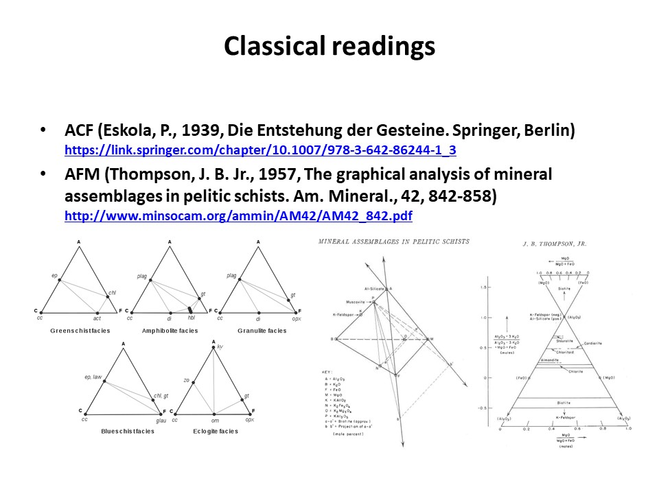
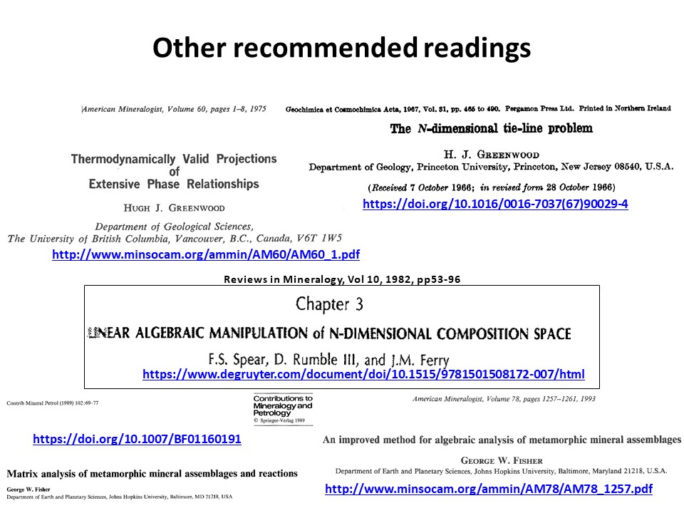
Greenwood, 1975: http://www.minsocam.org/ammin/AM60/AM60_1.pdf
Greenwood, 1967: https://doi.org/10.1016/0016-7037(67)90029-4
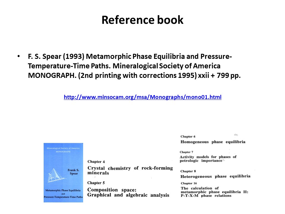
Spear et al., 1982: https://www.degruyter.com/document/doi/10.1515/9781501508172-007/html, or Spearetal1982
Fisher, 1989: https://doi.org/10.1007/BF01160191
Fisher, 1993: http://www.minsocam.org/ammin/AM78/AM78_1257.pdf

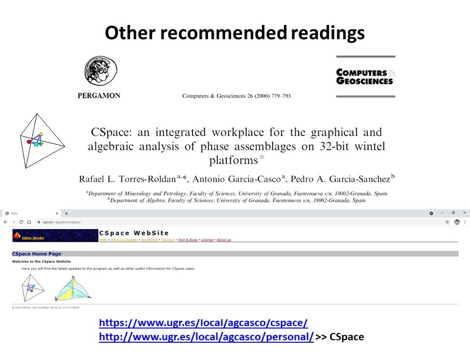
CSpace website: https://www.ugr.es/local/agcasco/cspace/
CSpace website: http://www.ugr.es/local/agcasco/personal/ >> CSpace

Torres-Roldan et al., 2000: https://doi.org/10.1016/S0098-3004(00)00006-6

"The student.... is urged... to concentrate on forming a mental image of the appearance of the composition space". Frank Spear, 1995.

See the crystal structure of almandine garnet (Fe3Al2Si3O12) in MINDAT database: https://www.mindat.org/min-452.html

Basic crystalchemistry of common minerals (in Spanish): https://www.ugr.es/~agcasco/personal/Cristalquimica/Cristalquimica.htm

MINDAT: https://www.mindat.org/

WEBMINERAL: http://www.webmineral.com/

Handbook of Mineralogy: http://www.handbookofmineralogy.org/index.html

IMA Reports published in the American Mineralogist

Nomenclature of the garnet supergroup, 2013
Edward S. Grew et al. pdf (2.3 MB)

Nomenclature of the amphibole supergroup, 2012
Frank C. Hawthorne et al. pdf (4.6 MB)

Named Amphiboles: A new category of amphiboles recognized by the International Mineralogical Association (IMA) and a defined sequence order for the use of prefixes in amphibole names, 2005
Ernst A.J. Burke And Bernard E. Leake pdf (84 KB)

Nomenclature of amphiboles: Additions and revisions to the International Mineralogical Association's amphibole nomenclature, 2004
Bernard E. Leake et al. pdf (188 KB)

IMA Reports prior to 1998 published in the Canadian Mineralogist

Robert F. Martin, editor The Canadian Mineralogist, has kindly let the Mineralogical Society of American host a set of International Mineralogical Association Commission on New Minerals and Mineral Names reports that were compiled by the Mineralogical Association of Canada and the Canadian Mineralogist on the occasion of the IMA 17th General Meeting in Toronto (August 1998). These reports are also available at the Mineralogical Association of Canada both as an electronic version and as a Booklet.

On the use of names, prefixes and suffixes, and adjectival modifiers in the mineralogical nomenclature, 1980
M.H. Hey and G. Gottardi pdf (176 KB)

The definition of a mineral, 1995
E.H. Nickel pdf (264 KB)

Formal definitions of type mineral specimens, 1987
P.J. Dunn and J.A. Mandarino pdf (236 KB)

Solid solutions in mineral nomenclature, 1992
E.H. Nickel pdf (324 KB)

Nomenclature of the micas, 1998
M. Rieder et al. pdf (412 KB)

Nomenclature of amphiboles: report of the Subcommittee on Amphiboles of the International Mineralogical Association, Commission on New Minerals and Mineral Names, 1997
B.E. Leake et al. pdf (1.2 MB)

Nomenclature of pyroxenes, 1989
N. Morimoto et al. pdf (1.5 MB)

Recommended nomenclature for zeolite minerals: report of the Subcommittee on Zeolites of the International Mineralogical Association, Commission on New Minerals and Mineral Names, 1997
D.S. Coombs et al. pdf (340 KB)

Classification and nomenclature of the pyrochlore group, 1977
D.D. Hogarth pdf (1.0 MB)

Nomenclature of platinum-group-element alloys: review and revision, 1991
D.C. Harris and L.J. Cabr /i pdf (1.1 MB)

Appendix. Symbols of the rock-forming minerals
After Kretz and Spear pdf (140 KB)

Mineral abbreviations:

IMA (pdf).

Kretz (1983, Am Min; html edited by A. Garcia-Casco)

Donna L. Whitney y Bernard W. Evans (2010; html edited by A. Garcia-Casco)

Also:

American Mineralogist Crystal Structure Database

IMA Mineral List with Database of Mineral Properties

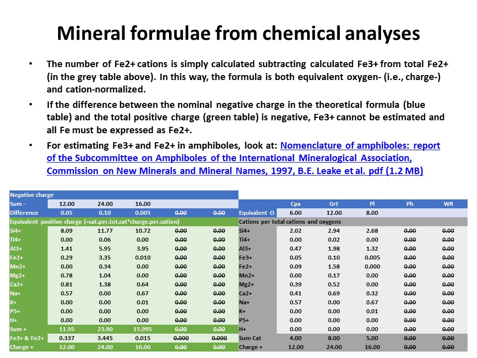
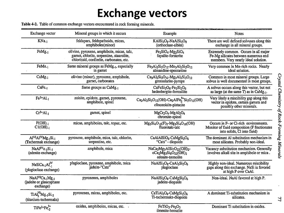
Solid solutions, end-members and exchange vectors

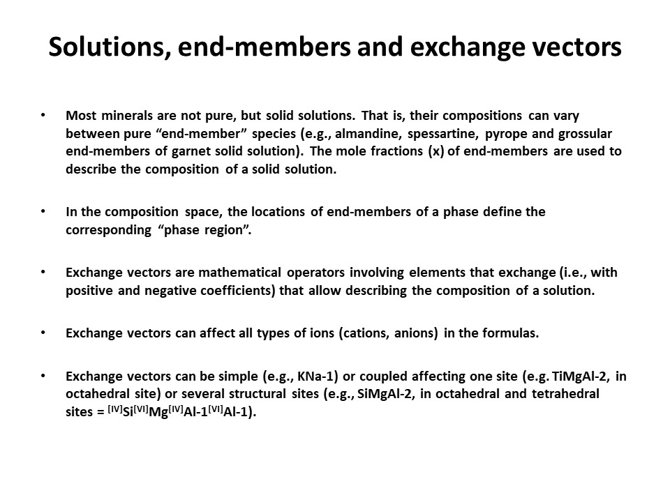
Exchange vectors: Mathematical operators (vectors) that allow describing the changes in chemical composition of a phase. They can be simple (e.g. KNa_-1, MgFe_-1) o coupled (CaAlNa_-1Si_-1, ^IVAl^VIAlMg_-1Si_-1), and involve cations, anions (Cl(OH)_-1) and vacant sites (^VIMg₃^VIAl_-2^VI(o)_-1, ^ANa^IVAl^A(o)_-1^IVSi_-1). They may hence not maintain a mass-balance (equal number of cations+anions in both sides of the vector, but they must maintaing electrostatic balance (equal number of charges in both sides of the vector). The exchange vectors normally work in more than one phase (e.g., micas, amphiboles, pyroxenes, chlorite, etc. etc.) and describe large groups of phases, in particular solid solutions with limited (partial) solution between them (e.g., dioctaedral and trioctaedral micas: ^VIMg₃^VIAl_-2^VI(o)_-1). They can be applied to any phase, including solids, liquids, gasses and fluids. When applied to solid solutions, the exchange vectors inform on their cristalchemical behavior because they contain structural information (for example, their formulation distinguishes ^IVAl from ^VIAl or ^ANa from ^BNa).

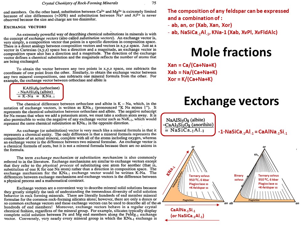
The formulations of exchange vectors are obtained subtracting two chemical species that represent end-members (or members, in general) of the solid solutions. This is shown below for the feldspars.

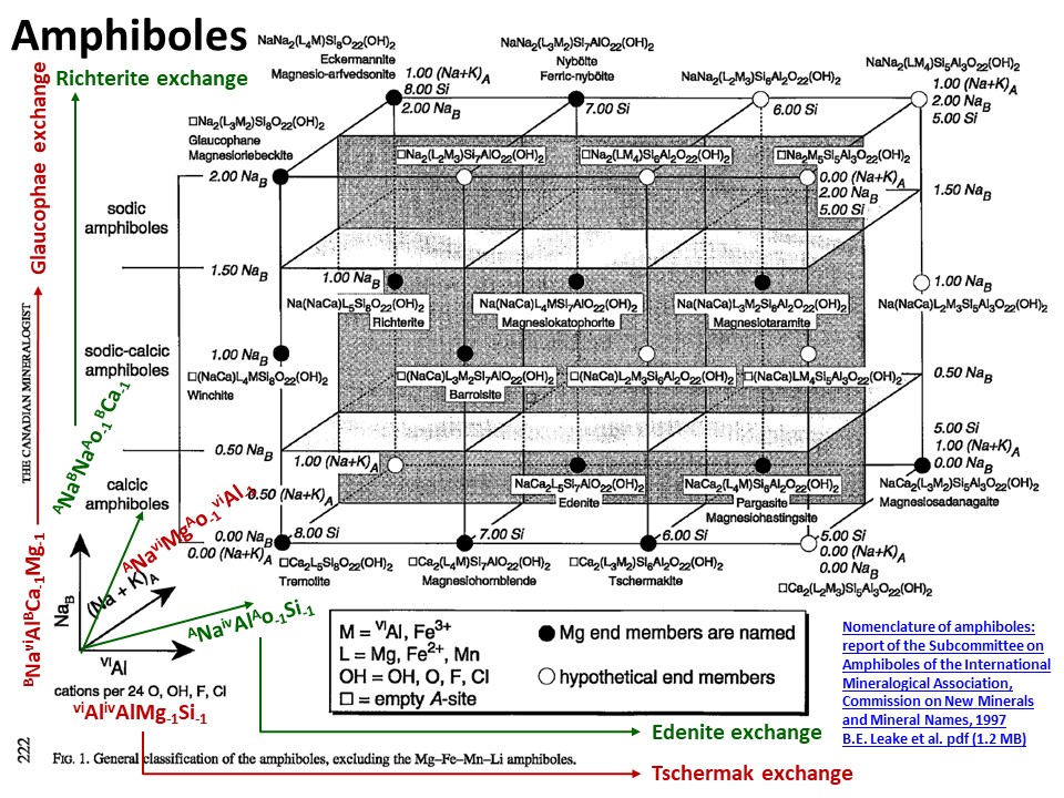
From: Bernard E. Leake; Alan R. Woolley; Charles E. S. Arps; William D. Birch; M. Charles Gilbert; Joel D. Grice; Frank C. Hawthorne; Akira Kato; Hanan J. Kisch; Vladimir G. Krivovichev; Kees Linthout; Jo Laird; Joseph A. Mandarino; Walter V. Maresch; Ernest H. Nickel; Nicholas M. S. Rock; John C. Schumacher; David C. Smith; Nick C. N. Stephenson; Luciano Ungaretti; Eric J. W. Whittaker; Guo Youzhi. Nomenclature of amphiboles; report of the subcommittee on amphiboles of the International Mineralogical Association, Commission on New Minerals and Mineral Names. The Canadian Mineralogist (1997) 35 (1): 219–246. (https://pubs.geoscienceworld.org/canmin/article-lookup/35/1/219 or http://www.minsocam.org/MSA/IMA/ima98(11).pdf).

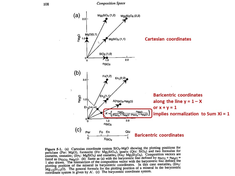
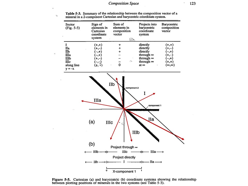
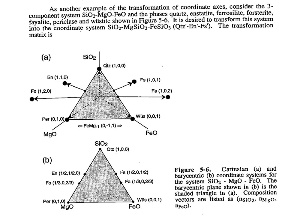
Composition space

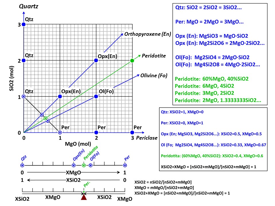
A simple chemical system with 2 dimensions: SiO2-MgO. Relations between cartesian and baricentric projections. The baricentric projection of a mineral vector (o the vector corresponding to any chemical species that can be fully described by the system) is found normalizing to 1:

XSiO2 = nSiO2/[nSiO2+nMgO]

XMgO = nMgO/[nSiO2+nMgO],

where nSiO2 and nMgO correspond to the cartesian molar values of SiO2 and MgO and XSiO2 and XMgO are termed mole fractions. In this normalization Sum Xi = 1.

The mole fractions, or the baricentric molar values of SiO2 and MgO, represent the intersection of two lines in the cartesian space. One line describes the mineral vector (y = a·x), while the other one describes the locus of the baricentric projection, which is defined as y = 1-x, or y+x = 1.

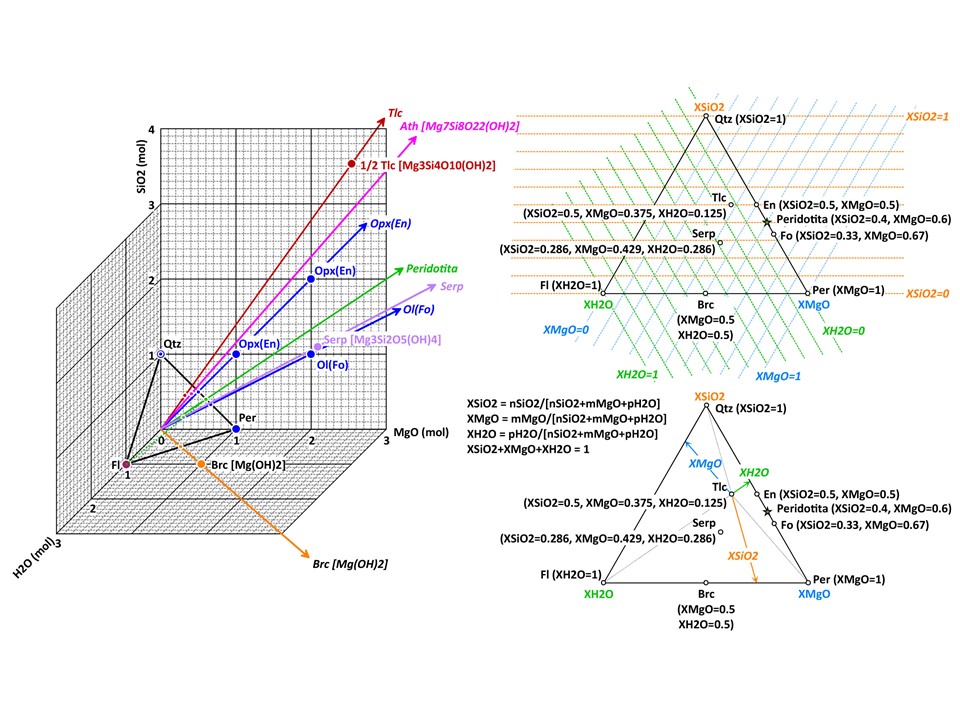
The same rules apply to any chemical system with n dimensions. Due to normalization, 2 independent cartesian variables transform into 1 independent baricentric variable, hence allowing the baricentric representation along a 1D line; 3 = 2D plane; 4 = 3D volume; 5, 6,... hyperplanes that cannot be fully represented, but can be represented after reducing the dimension of the baricentric space after condensation and projection (this is treated below).

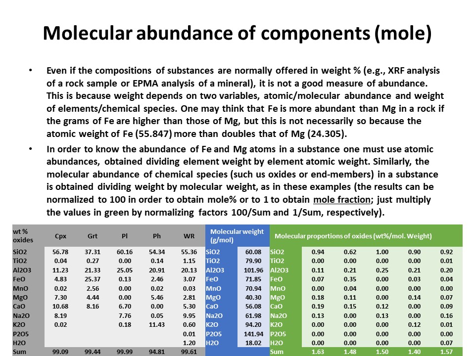
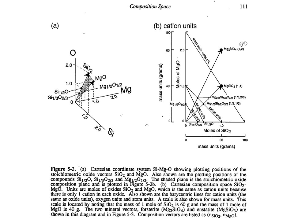
Units of measure. In general, the most commonly used in metamorphic petrogenesis are moles of oxides. Note, however, that oxide mass units (wt%) are commonly used in diagrams involving silicate liquids. In both cases, for historical reasons. Other interesting units of measure when dealing with oxygen-based components are oxygen (or oxyequivalent) units, useful for getting an idea of volume, rather than molecular, abundances of phases (because oxygen is the largest ion in aluminum-silicates). However, here we will use moles of oxides only.

Variations in the baricentric projection as a function of units of measure.

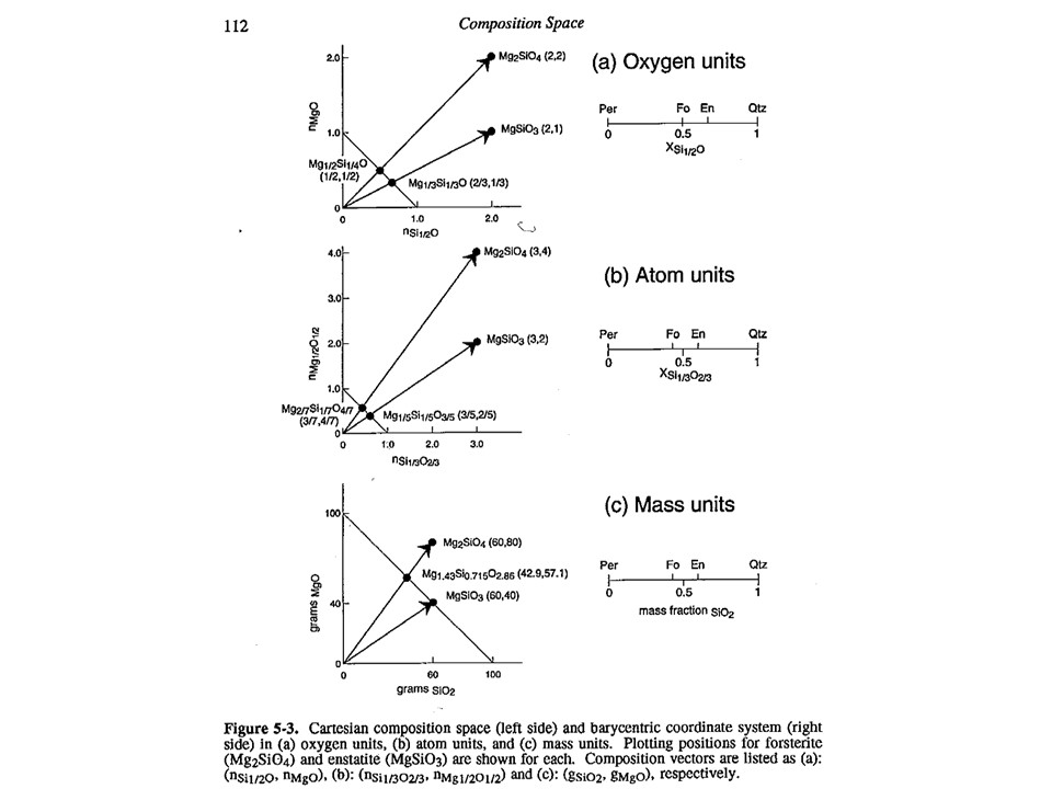
More on oxide molar units in 2 and 3 components systems (4 and higher component systems are explored below in this document).

Two components:

Three components:

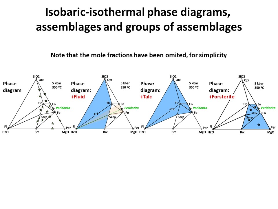
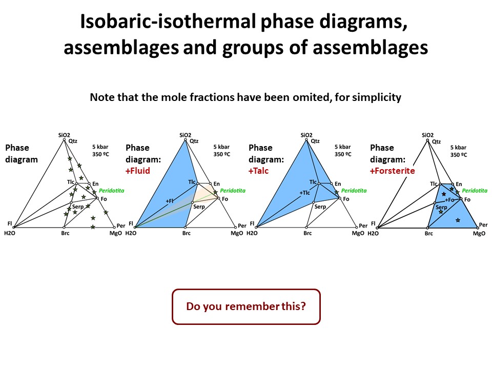
Three components: Phase diagrams with emphasis in subsets of associations that share a phase (examples in blue below: fluid, talc, olivine). In these examples, the coexisting minerals are joined by tie-lines (defining tie-triangles that describe the stable mineral associations under fixed P-T conditions) and the stars correspond to the composition of the system (= whole rock composition).

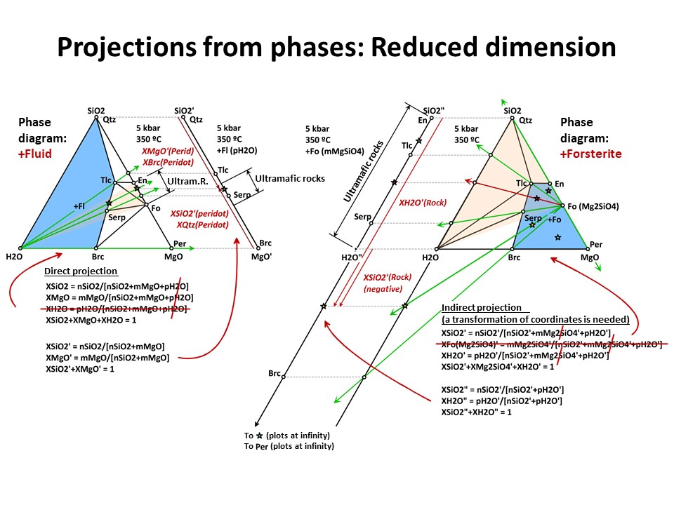
Projections 1

In a given system (say, a 3-component system represented in a baricentric 2D plane), one can project minerals and rocks from a given phase onto a part of the system. In doing this, only the corresponding subset of phase assemblage that share the projection phase can be projected (examples below, projection from fluid and olivine). This technique allows reducing the dimension of the represented baricentric space (which is mandatory when dealing with systems defined by a large number of chemical variables, as will be shown below in this document), but information is lost in the process because only a given subset of phase assemblages are represented in the projected baricentric space. The information on the amount of the projection phase is also lost.

The exercise is simple when the projection phase matches the composition of a component of the system (e.g., quartz = SiO2, periclase = MgO, fluid = H2O). For the last case, for example, the join (side) SiO2-MgO of the full SiO2-MgO-H2O triangle can receive the projection. In this case, the new mole fractions (XSiO2' and XMgO') are calculated excluding nH2O in the normalization formulas. This is because the projection from H2O does not impact in the amounts of nSiO2 (= nSiO2') y nMgO (= nMgO') of the projected chemical species. The same holds for projections from quartz (onto MgO-H2O join) or periclase (onto the SiO2-H2O join), which respective mole fractions are calculated excluding nSiO2 or nMgO, respectively).

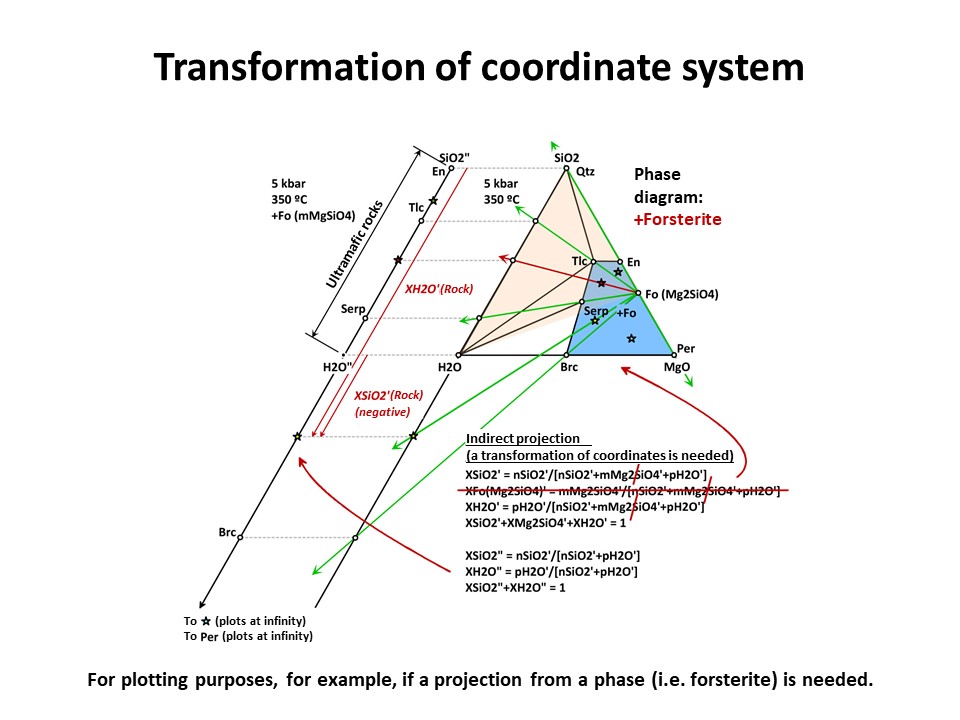
But the exercise is not son simple when the projection phase is more complex. Besides graphical solutions such as the right side diagram of the following figure, which represents a projection from olivine (forsterite) onto the SiO2-H2O join, a quantitative method is generally needed for calculating the new mole fractions (XH2O" y XSiO2") because no longer the procedure involves normalization using the original chemical variables. (-> see coordinate transformation, treated below). It must be noted that, for any species with SiO2+MgO, the projection from forsterite (that bears SiO2+MgO in the proportion 1:2) implies that nSiO2" and nMgO" do not equal nSiO2 y nMgO in the species. The latter must be corrected before normalization "discounting the amounts of forsterite in the species" in the proportion SiO2:MgO = 1:2. For this reason, the values of XSiO2" of some species are negative (i.e., plot at the negative sector of SiO2", away the locus of H2O", in the SiO2"-H2O" join) and even some species (such as periclase) plot at infinity (away the locus of H2O"), as shown in the figure. This problem will be treated quantitatively below. Meanwhile, we will inspect the graphical solution shown below in detail.

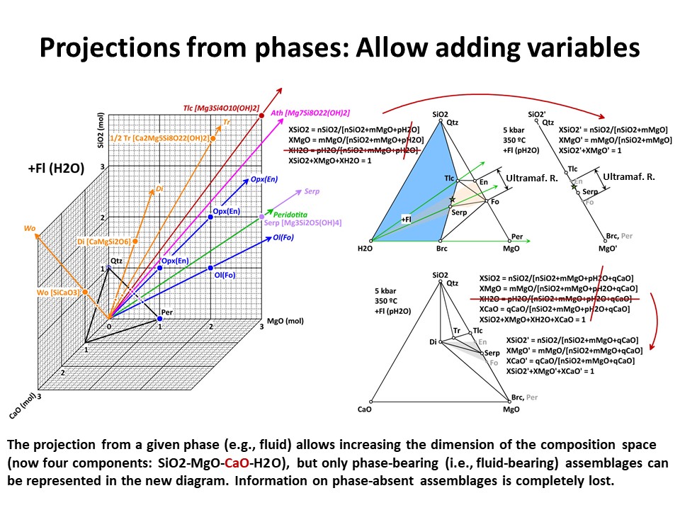
The projection of phases and rocks from a phase on a given subsystem (e.g., join) allows considering the graphical representation of larger systems, making the representation be closer to natural systems, but only under the limiting condition that all the projected assemblages must contain the projection phase. The assemblages that do not contain the projection phase H2O fluid in the following figure have been drawn in grey. In the case illustrated below, the system enlarges up to 4 components: SiO2-MgO-CaO-H2O. Because it is projected from H2O fluid, the simplest new ternary diagram MgO-SiO2-CaO (the composition of ultramafic rocks are represented by the grey shaded region defined by Fo-En-Di in the ternary diagram MgO-SiO2-CaO):

In the former case, the calculation of the new mole fractions is simple because the composition of the projection phase matches the composition of one of the chemical components that define the system. But, as above, this is not so in case of projections from complex phases, like forsterite (-> Coordinate transformation).

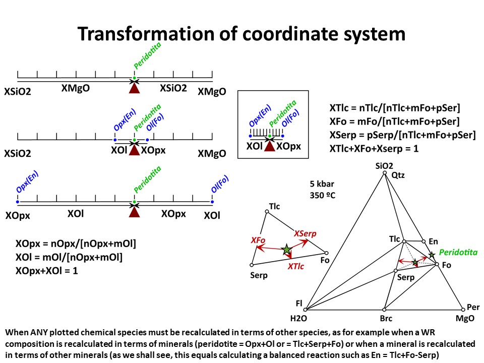
Coordinate transformation is needed for many other purposes (not only the graphical representation of systems with increased number of components). For example, the calculation of the (molar) abundance of minerals (or, in general, species) in a rock. Below, you will find examples in binary a ternary systems though, again, the principles are identical for n-dimension systems. The question is: Provided that we now the composition olivine (forsterite), orthopyroxene (enstatite) and a peridotite in the SiO2-MgO system, how much olivine and orthopyroxene does the peridotite have? Provided that we now the composition olivine (forsterite), talc, serpentine and an hydrated peridotite in the SiO2-MgO-H2O system, how much olivine, talc, serpentine does the peridotite have at 350 ºC and 5 kbar?

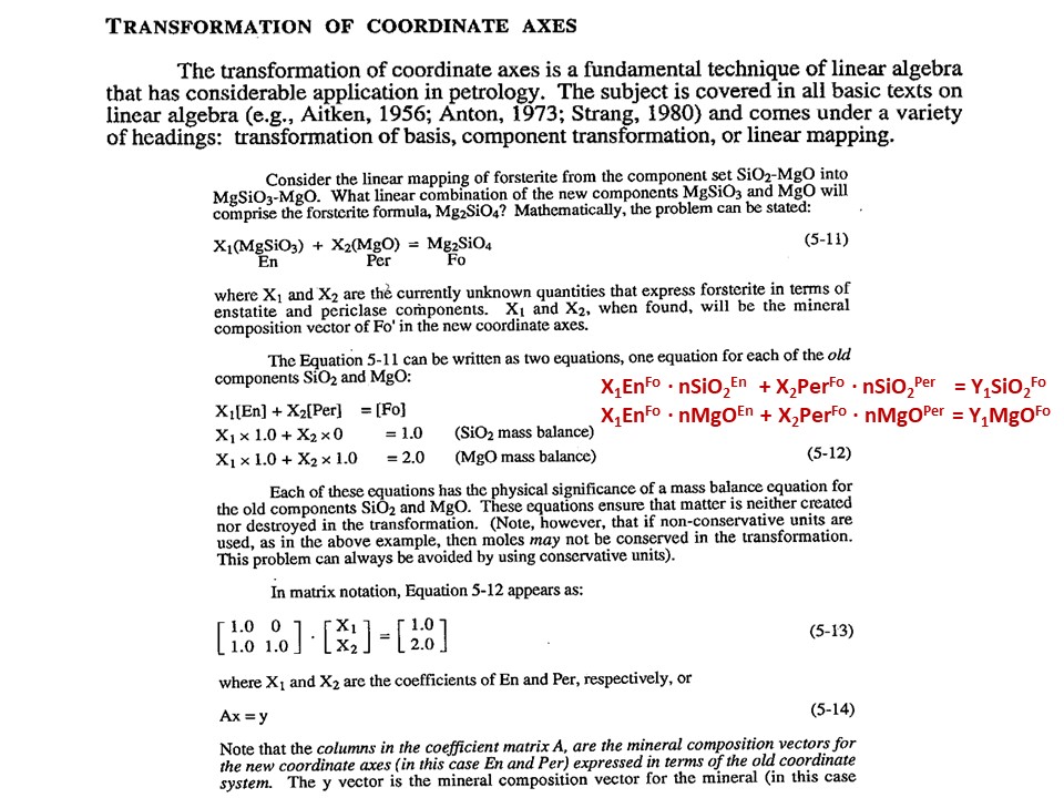
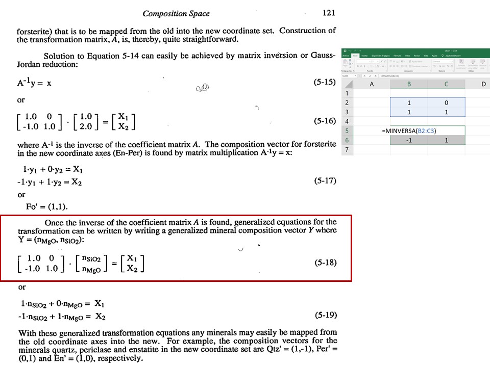
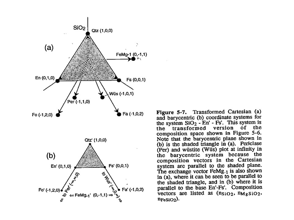
Coordinate transformation

Coordinate transformation is a rather common algebraic problem that make use of matrix calculus. Coordinate transformation has many applications in Mineralogy, Petrology and Geochemistry. It is known as "base transformation", "component transformation" or "lineal mapping".

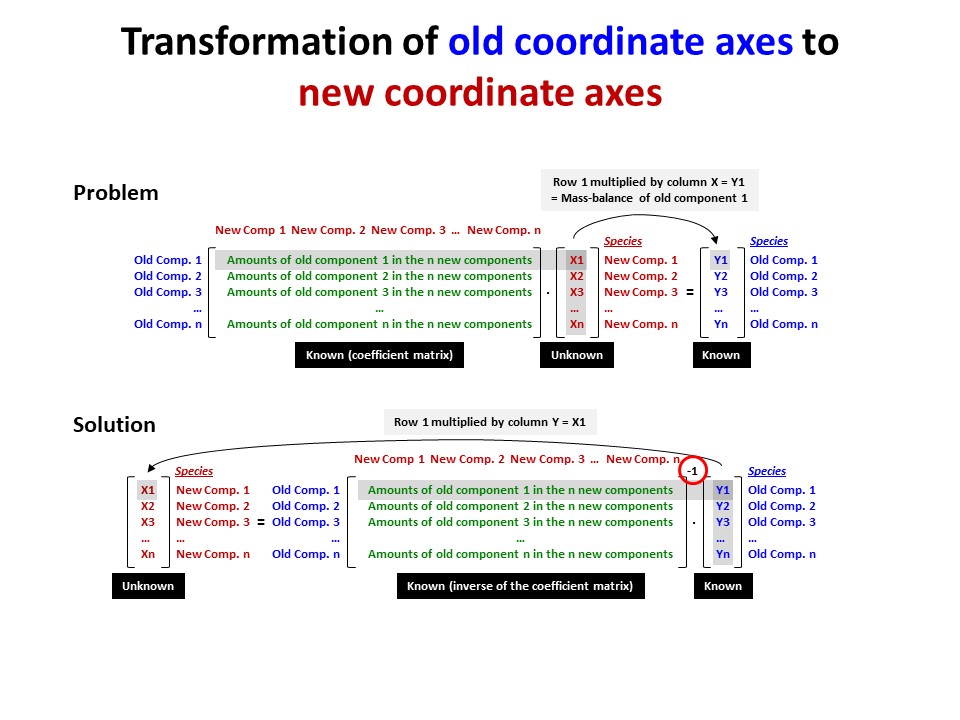
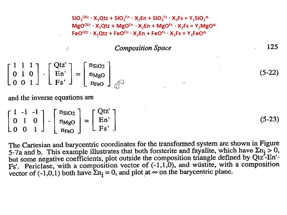
* The issue is to express a chemical species (mineral, rock, fluid, melt...) in terms of a set of new components given its known composition in terms of a set of old components. This can be achieved solving a set of linear mass-balance equations. As a general rule, the number of old and new components and, hence, the number of equations, must be equal. In the set of equations, there is a mass-balance per old component, so that the structure of the equations is regular and can be represented as in matrix notation, as below using matrix inversion among a number of ways of solving the set of equations.

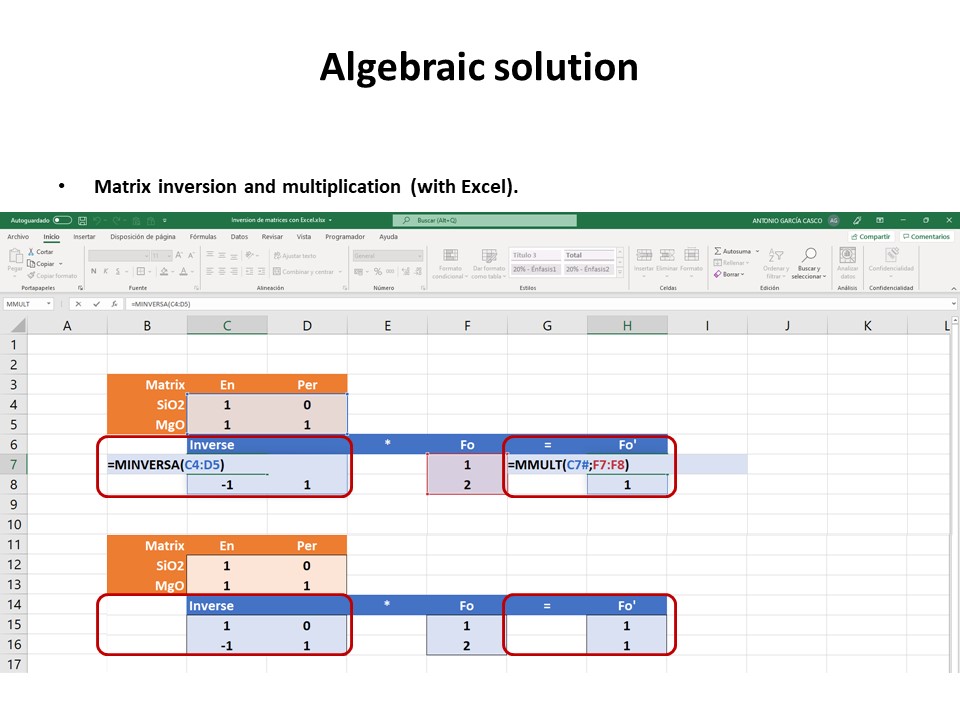
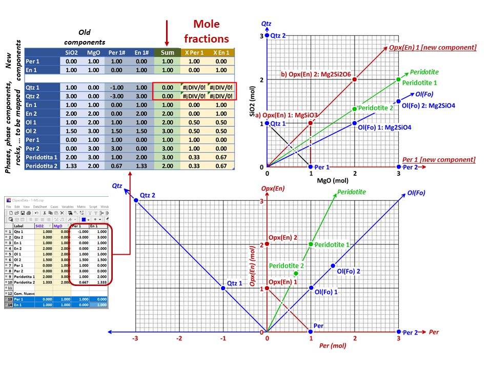
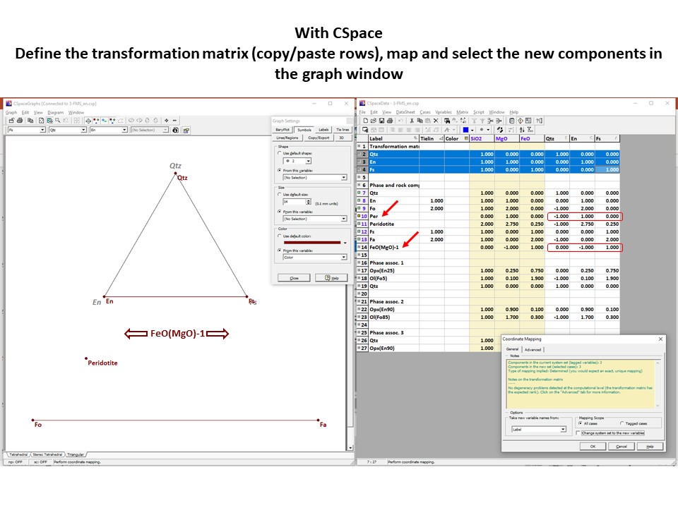
Let's consider the issue in the simple SiO2-MgO system.

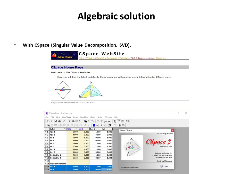
Or click here: 1-MS.csp

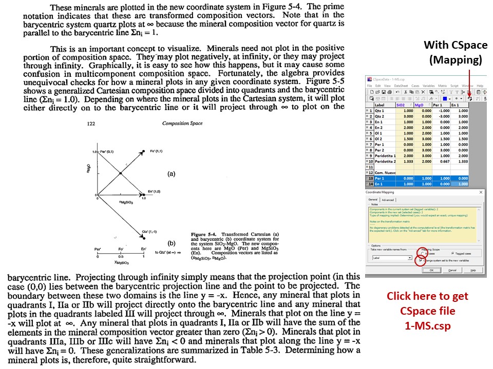
Coordinate transformation: SiO2-MgO -> En(SiMgO3)-Per(MgO). Note that quartz projects at infinity (that is, it cannot be projected) in the new coordinate system.

Coordinate transformation: SiO2-MgO -> En(Si2Mg2O6)-Per(MgO). Note that quartz projects at infinity (that is, it cannot be projected) in the new coordinate system, but it can be projected through infinity with a negative value of XEn (that is, it can be projected in the negative sector of XEn)

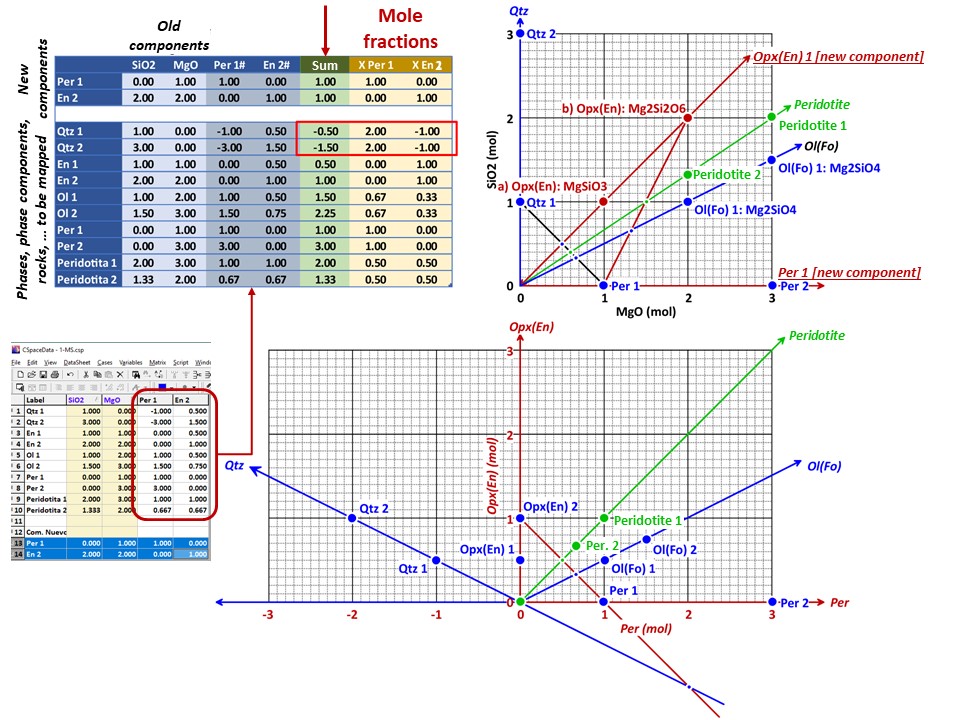
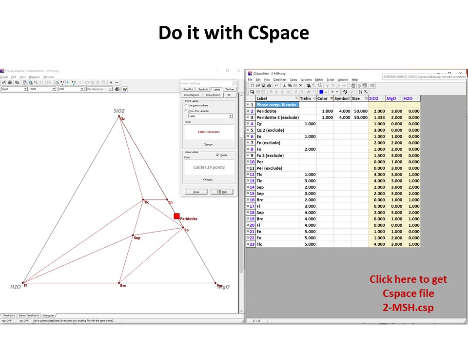
Or click here: 2-MSH.csp

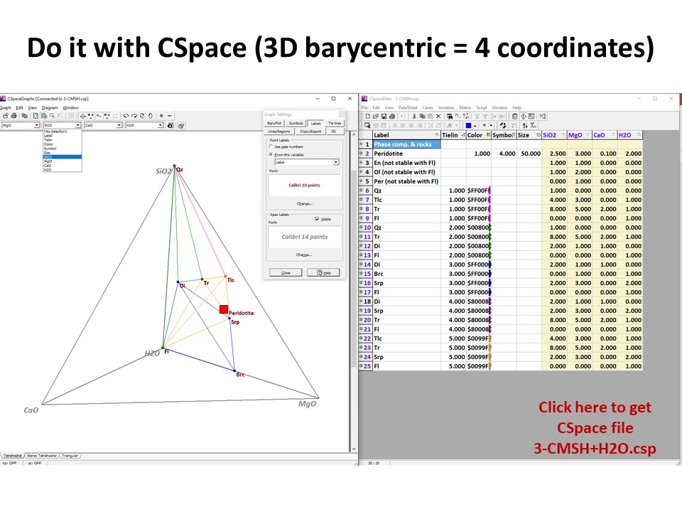
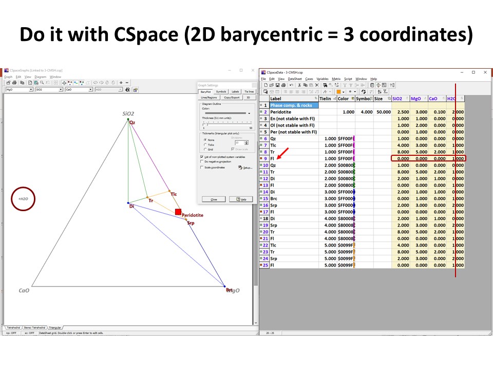
Or click here: CMSH+H2O.csp

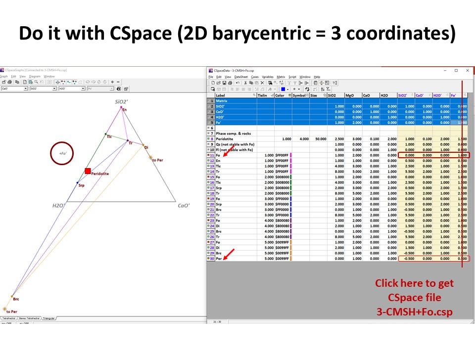
Or click here: 3-CMSH+Fo.csp

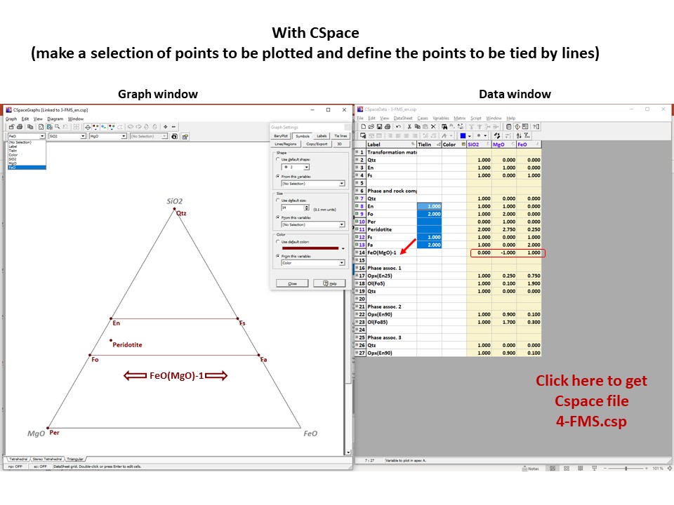
Or click here: 4-FMS.csp

Projection and condensation of the system

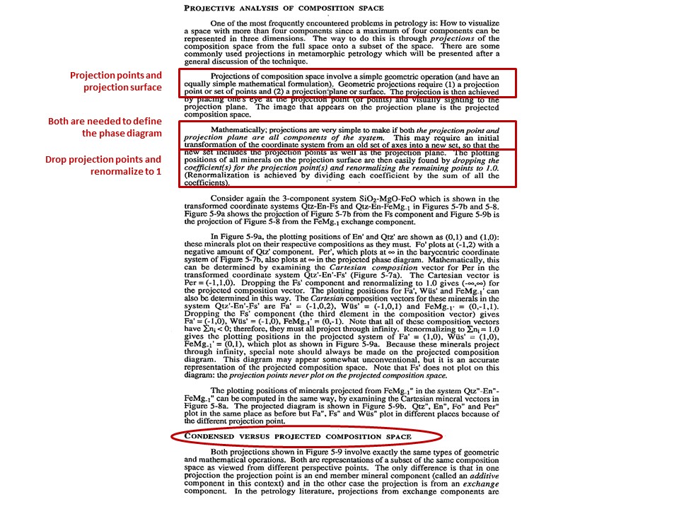
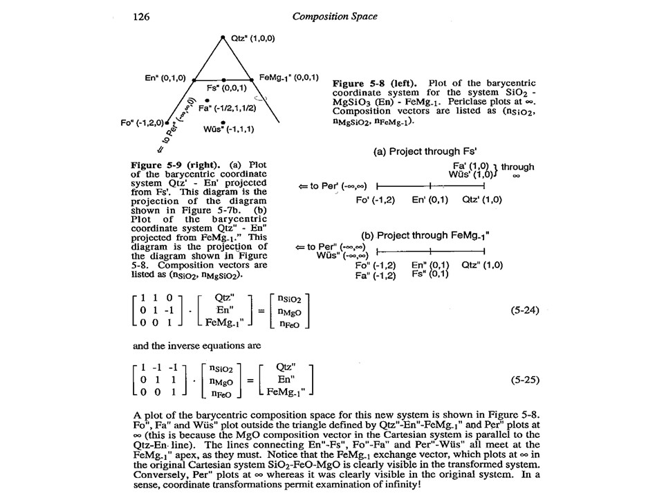
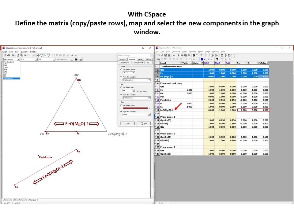
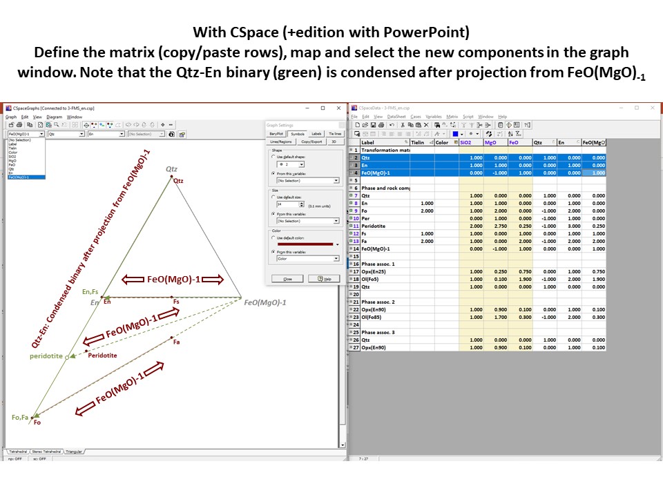
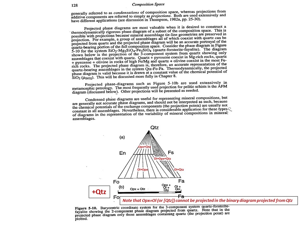
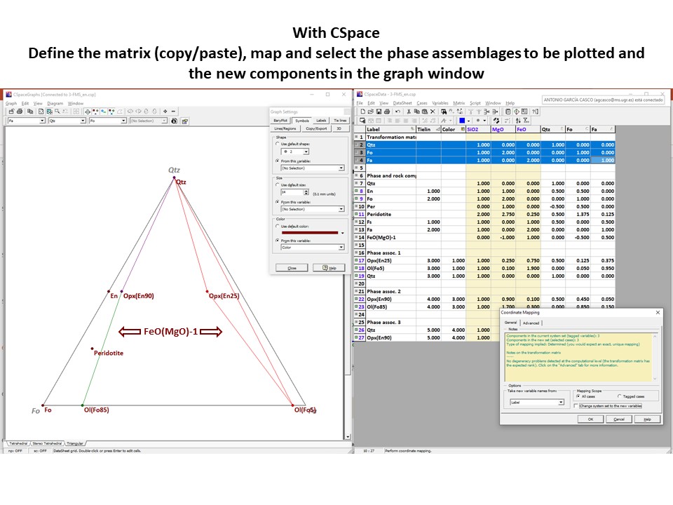
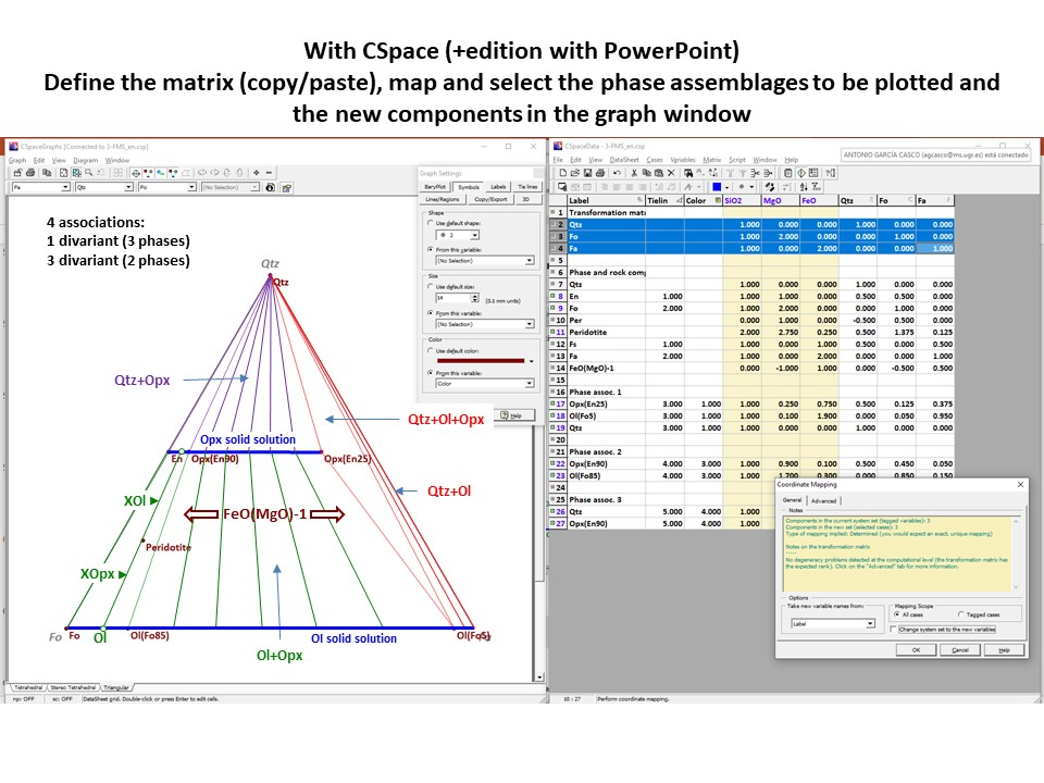
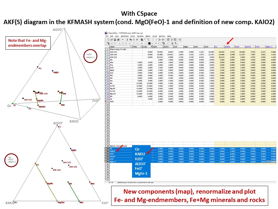
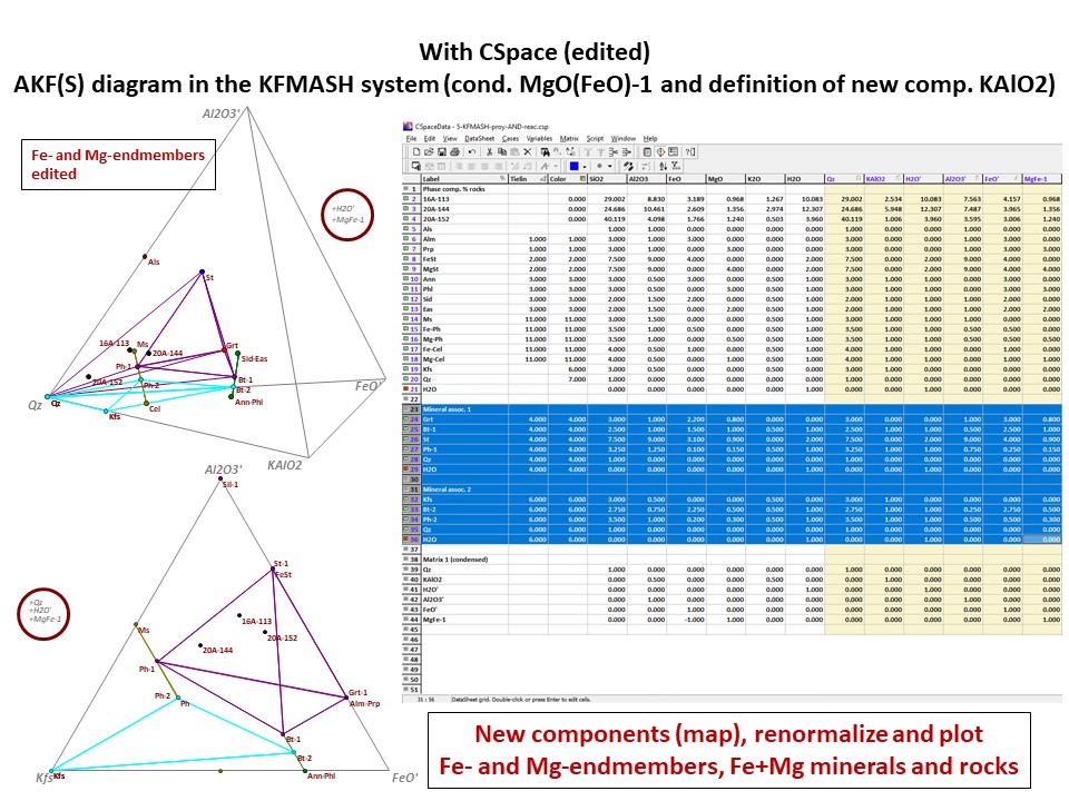
Diagrama AKF

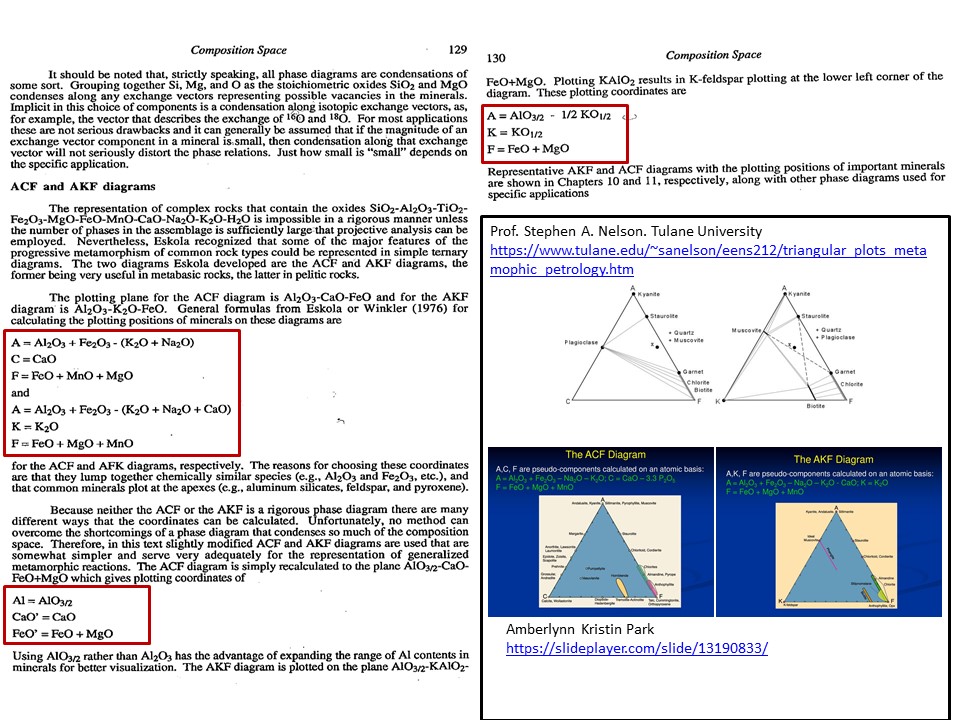
Prof. Stephen A. Nelson. Tulane University: https://www.tulane.edu/~sanelson/eens212/triangular_plots_metamophic_petrology.htm

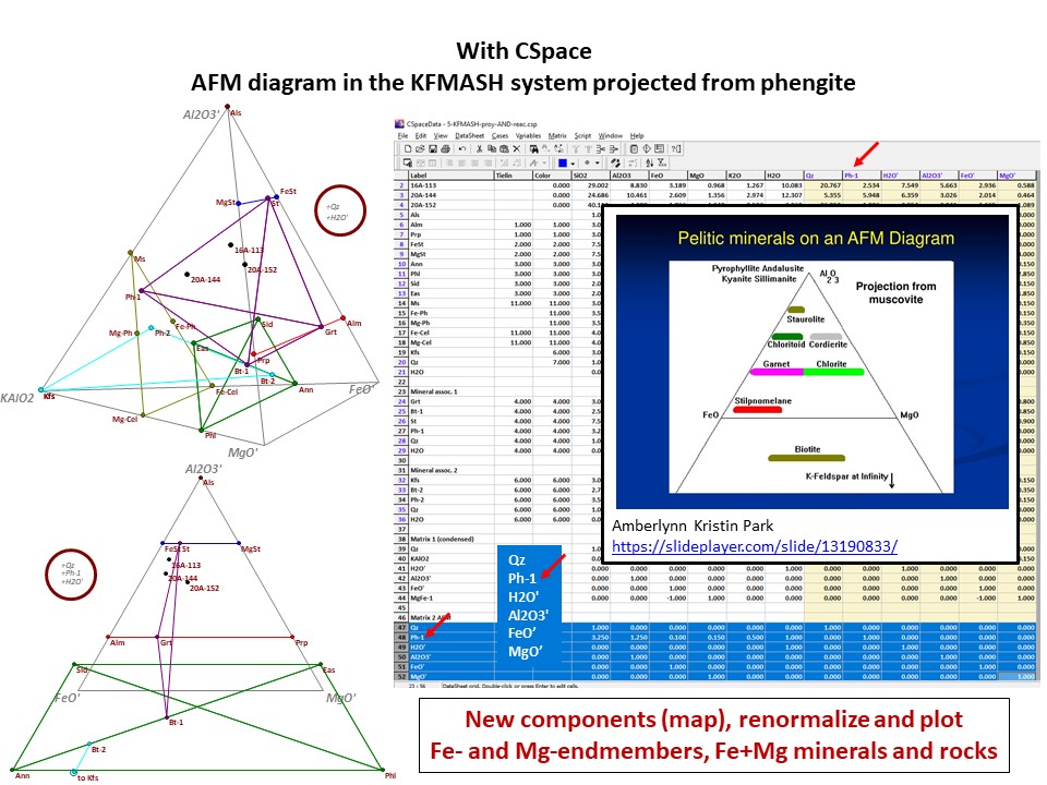
Amberlynn Kristin Park: https://slideplayer.com/slide/13190833/

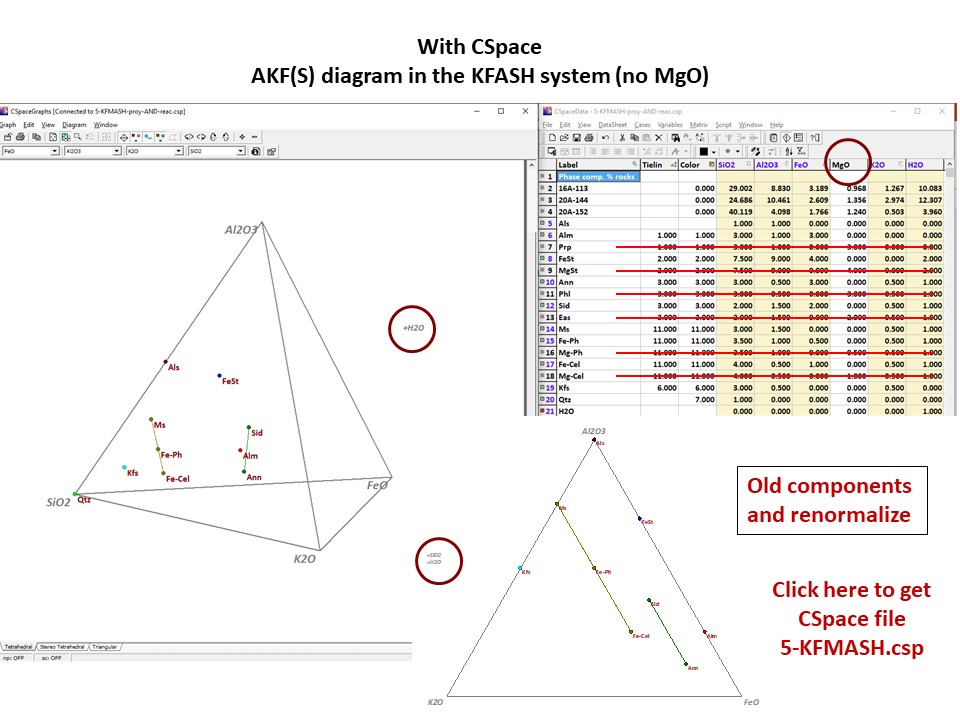
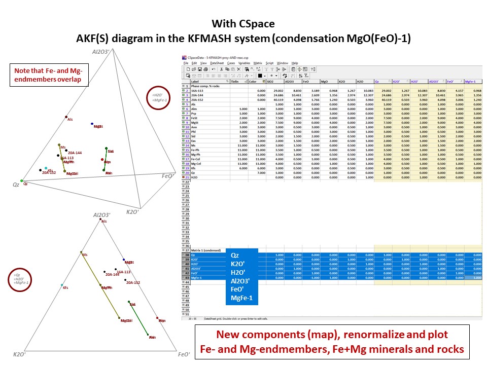
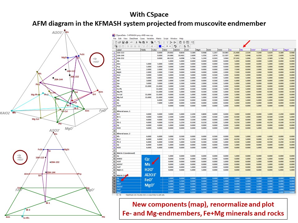
Or click here: 5-KFMASH.csp

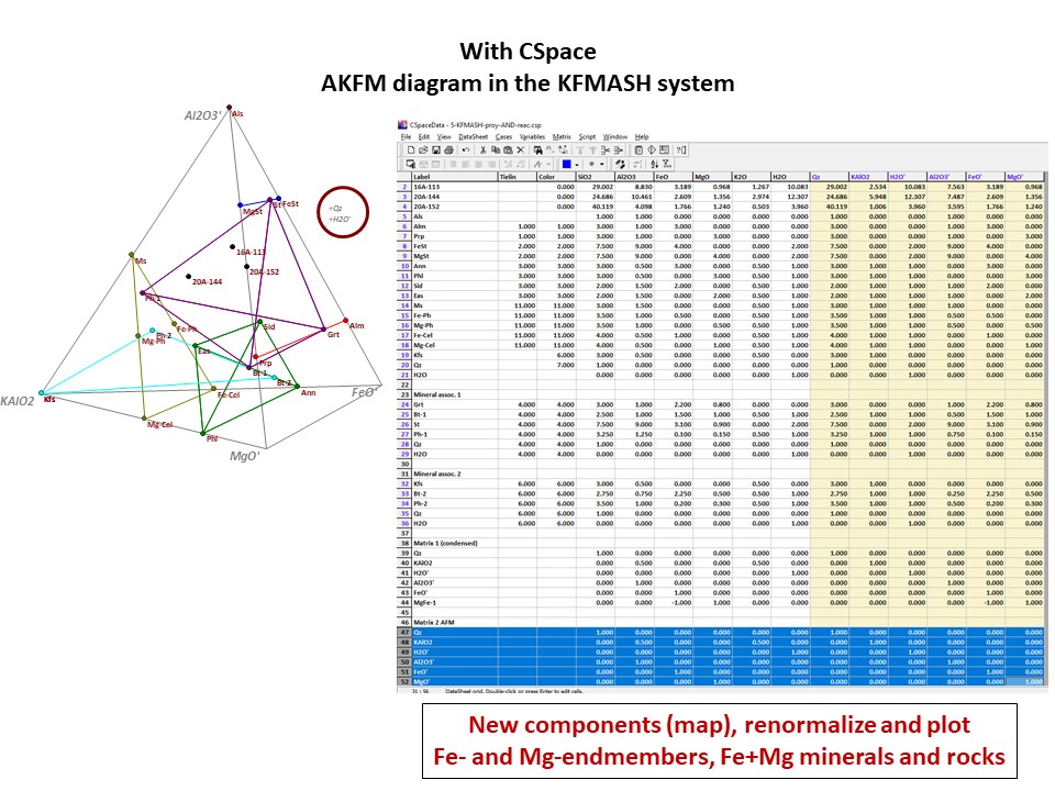
AFM diagram

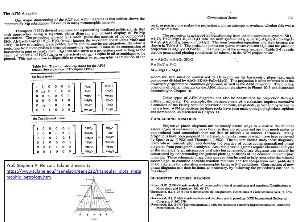
Prof. Stephen A. Nelson. Tulane University: https://www.tulane.edu/~sanelson/eens212/triangular_plots_metamophic_petrology.htm

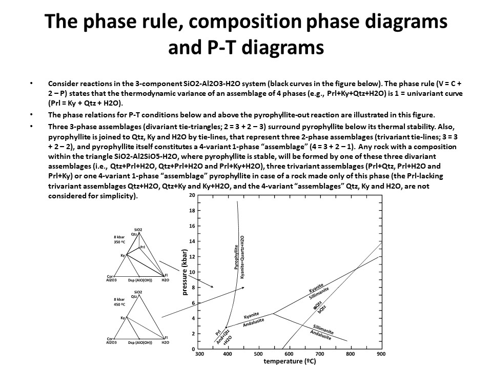
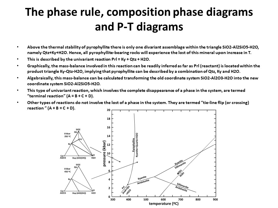
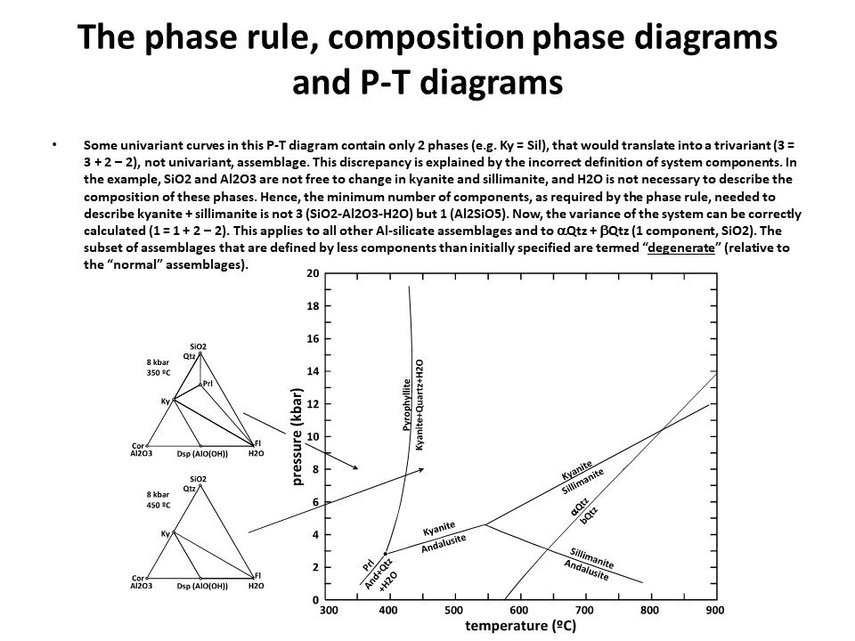
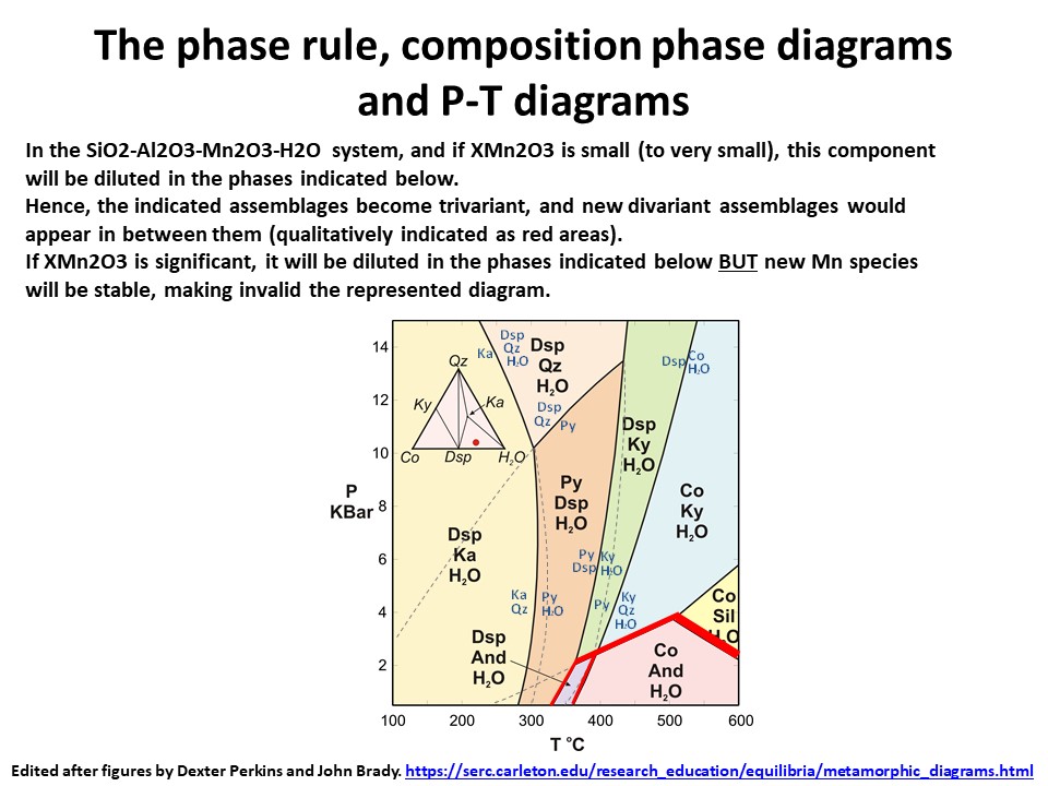
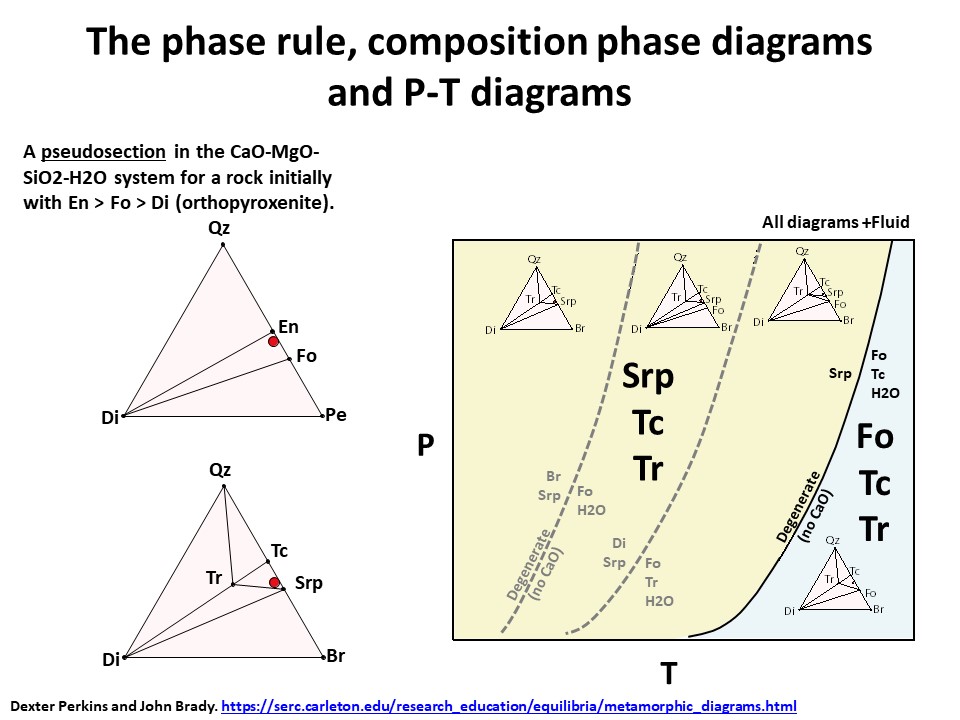
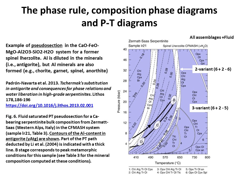
The phase rule, composition phase diagrams and P-T diagrams

* Number of components + 2 - number of coexisting phases (phase assemblage) equals the thermodynamic variance (or degrees of freedom) of the phase assemblage.

Advanced Petrology @ IPGP. Composition and P-T phase diagrams

Última modificación: viernes, 03 de febrero de 2023 15:23 +0100