|
Network Analysis Tool (download the code here: nat.c) Written in C, this program reads the adjacency matrix of a graph and returns various measures thereof regularly used in the study of complex networks. The input, which should be a text document, is assumed to define a simple undirected network, laid out as three columns (separations can be either tabs of spaces) representing: the label of one node, the label of another, and the value of the corresponding element of the adjacency matrix (zero if the two nodes are not linked, and one if they are). It doesn’t matter if the zero elements are not listed, since this is the default value. However, if, for instance, the input document lists only the nodes which are connected and no matrix elements, then one must go to line 152 of the program and make the appropriate changes in the reading of the data.
How to use nat.c Compilation requires linking the maths library. For example, in Linux, with the gcc compiler, this can be done by writing gcc nat.c –o nat.exe –lm in the console. If you prefer, you can also download an executable that should run on Linux platforms here. Say the input file is stuff.txt. To execute the program, write ./nat.exe stuff.txt. Three output text documents will then be created: sw_stuff.txt, p_stuff.txt and mix_stuff.txt. The first lists various measures relating to the input network, on different lines: · The mean degree <k> (average number of neighbours per node), the number of nodes N, and the standard deviation of the degree distribution (the degree of a node is its number of neighbours, or nodes connected to it by edges). · The clustering coefficient C (average over all the nodes i of Ci, which is the proportion of i’s neighbours which are mutually connected), its standard deviation, the expected value of C in the fully random graph model, C_rand, and the expected value of C in the configuration model, C_conf. [The fully random model is an imaginary network in which <k>N/2 edges are randomly placed among N nodes with no other constraints, yielding a Poissonian distribution of degrees. The probability that an edge exist between two nodes i and j is <k>/N. The configuration model is one in which the <k>N/2 edges are placed among the N nodes randomly but with the constraint that the degree distribution of the input network is conserved. The probability that an edge exist between nodes i and j is now kikj/(<k>N) (as long as ki, kj<<N) . By comparing a particular measure against the expected value in this null model, it is often possible to asses whether its value is simply the consequence of the network’s degree heterogeneity or some functional constraint must be looked for.] · The mean minimum path l (average over all pairs of nodes of the minimum number of edges linking the two), its standard deviation, the expected value in the fully random graph model, l_rand, and its expected value in the configuration model, l_conf. · The mean neighbour degree <knn> (average over all nodes of the average degree of each node’s neighbours) and the expected value in the configuration model, <knn>_conf (in the fully random model it is simply <knn>_conf=<k>, but when degree heterogeneity is taken into account the expected value is higher, since a randomly chosen node’s neighbourhood is no longer a representative sample of the network — more highly connected nodes appearing in more neighbourhoods than poorly connected ones). · Pearson’s correlation coefficient r (average over all pairs of connected nodes of the correlation between the degree of one and the other). Mark Newman suggested using this measure to asses the so-called mixing — or assortativity — by degree of complex networks. For a network with no degree-degree correlations, such as the fully random model or the configuration model, r=0. However, if the network is assortative — i.e., if highly connected nodes tend to be connected to other highly connected nodes — then r>0. If, on the other hand, it is disassortative, one in which highly connected nodes tend to have poorly connected ones for neighbours, then r<0. (Among real-world networks, social networks are usually assortative, while almost all other networks — technological, biological, linguistic — tend to be disassortative. Although this can often be understood for specific instances, the reason behind the general rule remains an open question in the field of complex networks.)
File p_stuff.txt contains the degree distribution, arranged in three columns: degree k, probability distribution p(k), and number of nodes with a given k, n(k).
File mix_stuff.txt has information on degree-degree correlations. The first column can be taken to represent either node labels or degrees; we’ll call a number in this column j. The second is the degree of node j, kj. The third is the mean degree of j’s neighbourhood — i.e., <knn>j=∑ikiaij/kj, where a is the adjacency matrix. The fourth, <knn(k)>, is the mean neighbour degree of nodes with degree k=j.
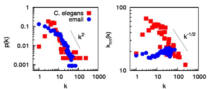
Example As an illustration, we use nat.c to study two different networks, the data for which can be found on Álex Arenas’ homepage: the network of e-mail interchanges between members of the Univeristy Rovira i Virgili (Tarragona) [R. Guimera, L. Danon, A. Diaz-Guilera, F. Giralt and A. Arenas, Phys. Rev. E 68, 065103(R) (2003)] and the network of metabolic reactions of the worm C. elegans [J. Duch and A. Arenas, Phys. Rev. E 72, 027104 (2005)]. The panel on the left of the figure shows the degree distributions (a plot of columns 1:2 of p_filename.dat), which are both highly heterogeneous and have tails that go roughly as p(k)~k-2. The panel on the right displays the degree-degree correlations (columns 1:4 of mix_filename.dat). While for the email network the value increases slightly with k (it is assortative), for the metabolic network it decreases approximately as <knn>~1/√k (it is disassortative).
The table below (found in sw_filename.dat), shows up two interesting differences between the social network and the biological one. They are both highly clustered (C~1) while their mean minimum paths are small [l~ln(N)], making them examples of small worlds. However, while the clustering coefficient of the e-mail network is nearly an order of magnitude greater than we should expect from its degree heterogeneity, that of the worm’s metabolic network, though larger in absolute terms, is less than twice the configuration-model value. This makes sense, since in social networks the friends of your friends are often also your friends, leading to a higher clustering, whereas in the metabolic network there is perhaps no such clustering mechanism — or it is less important.
The second difference is in the mixing. Whereas the social network is slightly assortative (r>0) — perhaps due to homophily or some such mechanism —, the biological one is strongly disassortative, as are most non-social networks for reasons which remain somewhat mysterious. [We have recently suggested that the “natural” or equilibrium state of networks is disassortative due to considerations of maximum entropy: Johnson et al., Phys. Rev. Lett. 104, 108702 (2010) (preprint | link)]
I hope this simple program may be useful to anyone who happens to have a network they would like to understand better. Please feel free to adapt and improve it wherever you want, and to write to me with any questions/remarks/suggestions/complaints… (well, perhaps not complaints) to
Thanks to Joaquín J. Torres for providing the codes for some of the functions. |
|
Home Research CV Publications Teaching Software Miscellanea Links Contact |
|
Home Research CV Publications Teaching Software Miscellanea Links Contact |
|
|
|
C. Elegans |
|
<k> |
9.62 |
8.97 |
|
N |
1133 |
453 |
|
σ |
9.34 |
16.74 |
|
C |
0.22 |
0.71 |
|
Crand |
0.0085 |
0.020 |
|
Cconf |
0.029 |
0.38 |
|
l |
3.60 |
2.66 |
|
lrand |
3.11 |
2.79 |
|
lconf |
2.66 |
2.07 |
|
<knn> |
17.90 |
51.56 |
|
<knn>conf |
18.69 |
40.24 |
|
r |
0.078 |
-0.22 |